Euler Method

Published on: May 13, 2024 at 6:00 PM

Euler Method applied for numerically solving Ordinary Differential Equations.

Written by: Andre Albano

To approximate Ordinary Differential Equations (ODEs) we normally use numerical methods and initial value problems. A typical IVP is given by:

\frac{\delta y}{\delta t} = f(y,\ t);\ a \le t \le b;\ y(a) = \alpha

Where $y(t)$ is what I want to approximate, $f(y,\ t)$ is a known function, $a$ and $b$ are the limits of the interval, and $\alpha$ is the initial condition.

There are several methods to solve ODEs numerically:

Euler
Taylor
Runge-Kutta
Runge-Kutta-Fehlberg
Adams-Bashforth
Adams-Moulton

And so on. The method covered in this post is the Euler Method.

The Euler method is a simple numerical method. It is based on the idea of approximating the solution of an ODE by a sequence of small steps. The method is named after the Swiss mathematician Leonhard Euler, who first introduced it in the 18th century.

It is based on the Taylor series expansion of the function $y(t)$ around the point $t_i$ :

y(t_{i+1}) = y(t_i) + (t_{i+1}-t_{i}) \cdot y'(t_i) + \frac{(t_{i+1}-t_{i})^{2}}{2}y''(\xi_{i})

For any $\xi_{i}$ in the interval $[t_i, t_{i+1}]$ . We can say that $(t_{i+1}-t_{i})$ is equal to the step size $h$ that is the element size. So, the Euler Method is:

y_{i+1} = y_i + h \cdot f(y_i,\ t_i)

Where $y_i$ is the approximation of $y(t_i)$ and $y_{i+1}$ is the approximation of $y(t_{i+1})$ . And both can be written as $\omega_i$ and $\omega_{i+1}$ respectively. So the formula can be written as:

\omega_{0} = y(t_{0}) = \alpha \\ \omega_{i + 1} = \omega_{i} + h \cdot f(\omega_{i}, t_{i})

The Euler method is a first-order method, which means that the error is proportional to the step size $h$ .

Example: Let’s solve the following ODE:

\frac{\delta y}{\delta t} = y - t^{2} + 1;\ 0 \le t \le 2;\ y(0) = 0.5 ;\ h = 0.2

First we have to analyze the value of the step size $h$ . The interval is $[0, 2]$ and the step size is $0.2$ , so we have 10 steps. The values of $t$ are:

t_0 = 0.0, t_1 = 0.2, t_2 = 0.4, t_3 = 0.6, t_4 = 0.8,

t_5 = 1.0, t_6 = 1.2, t_7 = 1.4, t_8 = 1.6, t_9 = 1.8

So that means that the number of iterations is equal to 10. What we have to do is, take the initial function $\frac{\delta y}{\delta t} = y' = y - t^{2} + 1 = f(\omega_i,\ t_i)$ and apply the Euler method to approximate the values of $y$ in each step. The initial condition is $y(0) = 0.5$ .

\omega_{0} = 0.5

\omega_{i + 1} = \omega_{i} + h \cdot (\omega_{i} - t_{i}^{2} + 1)

So $\omega_{0 + 1} = \omega_{1}$ for the first iteration is going to be:

\omega_{1} = 0.5 + 0.2 \cdot (0.5 - 0^{2} + 1) = 0.8

And the rest of iterations are:

\omega_{2} = 0.8 + 0.2 \cdot (0.8 - 0.2^{2} + 1) = 1.152

\omega_{3} = 1.152 + 0.2 \cdot (1.152 - 0.4^{2} + 1 = 1.5504

\omega_{4} = 1.5504 + 0.2 \cdot (1.5504 - 0.6^{2} + 1) = 1.9884

\omega_{5} = 1.9884 + 0.2 \cdot (1.9884 - 0.8^{2} + 1) = 2.4580

\omega_{6} = 2.4580 + 0.2 \cdot (2.4580 - 1.0^{2} + 1) = 2.9498

\omega_{7} = 2.9498 + 0.2 \cdot (2.9498 - 1.2^{2} + 1) = 3.4517

\omega_{8} = 3.4517 + 0.2 \cdot (3.4517 - 1.4^{2} + 1) = 3.9501

\omega_{9} = 3.9501 + 0.2 \cdot (3.9501 - 1.6^{2} + 1) = 4.4281

\omega_{10} = 4.4281 + 0.2 \cdot (4.4281 - 1.8^{2} + 1) = 4.8657

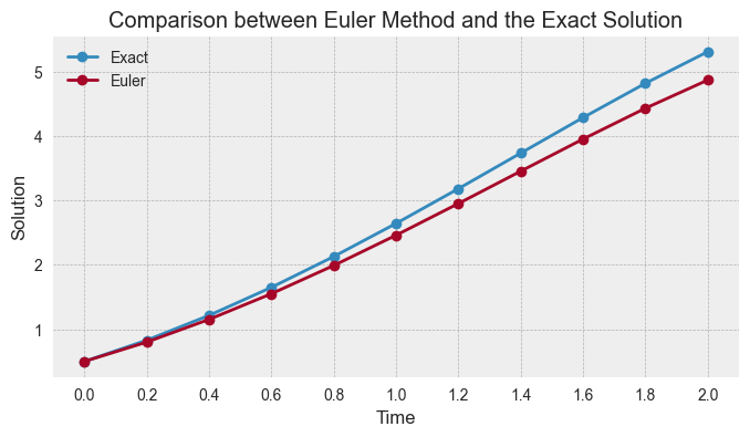
So the approximate value of $y(2)$ is $\omega_{10} = 4.8657$ . For comparison, the exact solution of the ODE is:

y(t) = t^{2} + 2t + 1 - 0.5e^{t}

So the exact value of $y(2)$ is:

y(2) = 2^{2} + 2 \cdot 2 + 1 - 0.5e^{2} = 5.3054

So the error of the Euler method is:

\text{Error} = |4.8657 - 5.3054| = 0.4397

The error is 0.4397, which is a good approximation for the Euler method.

Below we can see the plot of the exact solution and the Euler method approximation.

euler demonstration

And below, we can see the Python code that implements the Euler method for the ODE:

def euler(edo, a, b, h, y0):
    t = np.linspace(a, b, int(np.ceil(b-a)/h)+1)
    n = np.zeros(len(t))
    n[0] = y0

    for i in range(0, len(t)-1):
        k = edo(t[i], n[i])
        n[i+1] = n[i] + h * k

    return t, n

So, to sum up the Euler method is considered a simple method to approximate ODEs. The method is easy to implement and understand, but it is not very accurate. For more accurate methods, we can use the Runge-Kutta method or the Adams-Bashforth method.

André Albano @onablaerdna
I'm a Geophysicist and Coder. I work with seismic inversion algorithms, software development, well log analysis and so on.

Euler Method - ODEs