Runge Kutta Method

Published on: May 18, 2024 at 11:00 PM

Runge-Kutta methods (2nd, 4th order) for solving ordinary differential equations.

Written by: Andre Albano

One other method for solving Ordinary Differential Equations (ODEs) is the Runge-Kutta method. This method is a family of iterative methods that can be used to solve initial-value problems. The most common Runge-Kutta methods are the 2nd and 4th order.

The way to solve these methods are very similar to the Euler Method, but with more precision. The 2nd order Runge-Kutta method is also known as the midpoint method, and the 4th order Runge-Kutta method is the most commonly used.

The 2nd order Runge-Kutta method is given by:

w_{0} = \alpha \\ w_{i+1} = w_{i} + h f(t_{i} + \frac{h}{2}, w_{i} + \frac{h}{2} f(t_{i}, w_{i}))

And the 4th order Runge-Kutta method is given by:

w_{0} = \alpha \\ k_{1} = h f(t_{i}, w_{i}) \\ k_{2} = h f(t_{i} + \frac{h}{2}, w_{i} + \frac{k_{1}}{2}) \\ k_{3} = h f(t_{i} + \frac{h}{2}, w_{i} + \frac{k_{2}}{2}) \\ k_{4} = h f(t_{i+1} + h, w_{i} + k_{3}) \\ w_{i+1} = w_{i} + \frac{1}{6}(k_{1} + 2k_{2} + 2k_{3} + k_{4})

Yeah, it’s a lot. Let’s see an example and use the 4th Order Runge-Kutta Method, the same from the Euler Method:

y' = y - t^{2} + 1; \ 0 \le t \le 2;\ y(0) = 0.5;\ h = 0.2

The value of $h$ is the step size. The interval is $[0, 2]$ . So, we have 10 steps. The values of t are $t_{0} = 0.0,\ t_{1} = 0.2,\ t_{2} = 0.4, ...,\ t_{8} = 1.6,\ t_{9} = 1.8$

Just like the Euler Method, that means we have 10 iterations. Let’s begin the first two iterations

w_{0} = 0.5

In the first iteration $w_{i} = 0$ and $t_{i} = 0.0$

w_{1}: \begin{cases} K_{1} = 0.2 \cdot (0.5 - 0.0^{2} + 1);\ K_{1} = 0.3\\ K_{2} = 0.2 \cdot (0.5 + \frac{0.3}{2} - (0 + \frac{0.2}{2})^{2} + 1) ;\ K_{2} = 0.328 \\ K_{3} = 0.2 \cdot (0.5 + \frac{0.328}{2} - (0 + \frac{0.2}{2})^{2} + 1) ;\ K_{3} = 0.3308 \\ K_{4} = 0.2 \cdot ((0.5 + 0.3308) - (0.2)^{2} + 1) ;\ K_{4} = 0.3581 \\ \end{cases} \\ w_{1} = 0.5 + \frac{(0.3 + 2\cdot 0.328 + 2\cdot 0.3308 + 0.3581)}{6} = 0.8292

w_{2}: \begin{cases} K_{1} = 0.2 \cdot (0.8292 - 0.2^{2} + 1);\ K_{1} = 0.3578 \\ K_{2} = 0.2 \cdot (0.8292 + \frac{0.3578}{2} - (0.2 + \frac{0.2}{2})^{2} + 1) ;\ K_{2} = 0.3836 \\ K_{3} = 0.2 \cdot (0.8292 + \frac{0.3836}{2} - (0.2 + \frac{0.2}{2})^{2} + 1) ;\ K_{3} = 0.3862 \\ K_{4} = 0.2 \cdot ((0.8292 + 0.3862) - (0.4)^{2} + 1) ;\ K_{4} = 0.4111 \\ \end{cases} \\ w_{2} = 0.8292 + \frac{(0.3578 + 2\cdot 0.3836 + 2\cdot 0.3862 + 0.4111)}{6} = 1.2140

\vdots

w_{10}: \begin{cases} K_{1} = 0.2 \cdot (4.8150 - 1.8^{2} + 1);\ K_{1} = 0.5150 \\ K_{2} = 0.2 \cdot (4.8150 + \frac{0.5150}{2} - (1.8 + \frac{0.2}{2})^{2} + 1) ;\ K_{2} = 0.4925 \\ K_{3} = 0.2 \cdot (4.8150 + \frac{0.4925}{2} - (1.8 + \frac{0.2}{2})^{2} + 1) ;\ K_{3} = 0.4902 \\ K_{4} = 0.2 \cdot ((4.8150 + 0.4902) - (2.0)^{2} + 1) ;\ K_{4} = 0.4610 \\ \end{cases} \\ w_{10} = 4.8150 + \frac{(0.5150 + 2\cdot 0.4925 + 2\cdot 0.4902 + 0.4610)}{6} = 5.3053

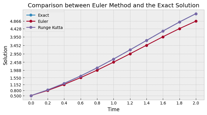
The final result is $y_{rk}(2) = 5.3053$ . If you recall the Euler Method result is

$y_{e}(2) = 4.8657$ .

It’s clear that the Runge-Kutta Method is more precise than Euler’s method. That’s because of its higher order of accuracy, which means it can provide a more accurate approximation of the solution over a given interval. It is designed to minimize the local truncation error, which is the error introduced at each step of the calculation. Also, higher order methods like this reduce the error more rapidly as the step size decreases.

When we compare to the exact values, the approximations we found on the Runge Kutta method have a very small error:

runge kutta demonstration

As we can see, the exact solution is overshadowed by the Runge Kutta method, showing it’s extremely small error.

Implementation

Below we have the implementation of 4th Order Runge Kutta method using Python.

import numpy as np

def runge_kutta(function, a, b, h, y0):
    t = np.linspace(a, b, int((b - a) / h) + 1)
    n = np.zeros(len(t))
    n[0] = y0

    for i in range(0, len(t) - 1):
        k1 = h * function(t[i], n[i])
        k2 = h * function(t[i] + h / 2, n[i] + k1 / 2)
        k3 = h * function(t[i] + h / 2, n[i] + k2 / 2)
        k4 = h * function(t[i + 1], n[i] + k3)

        n[i + 1] = n[i] + (k1 + 2 * k2 + 2 * k3 + k4) / 6

    return t, n

André Albano @onablaerdna
I'm a Geophysicist and Coder. I work with seismic inversion algorithms, software development, well log analysis and so on.